Predicting customer demand is crucial for growing business. Without reliable forecasts, we risk stockouts or excess inventory, leading to wasted resources. This is especially important for our wedding and event catering service, where we work with perishable ingredients. By precisely estimating daily and weekly demand, we can optimize inventory, reduce waste, control costs, and consistently meet customer expectations.
Before diving into forecasting, we’ll start with data exploration. This includes analyzing variable distributions, handling missing values, and uncovering key insights. For this analysis, we’ll use a dataset from Kaggle. You can explore it here: Kaggle - Food Demand Forecasting.
The data contains information from 77 stores over a period of 145 weeks.
Two types of promotions (web, email) were shown in the data as below:
- 10.61% stores ran one type of promotion.
- 4.21% stores ran both types at the same time.
- 85.18% stores didn’t run any promotions.
Our initial analysis is aim to discover:
(1) Did revenue or profit increase?
(2) Which promotion worked best?
(3) To predict future demand for our menu items.
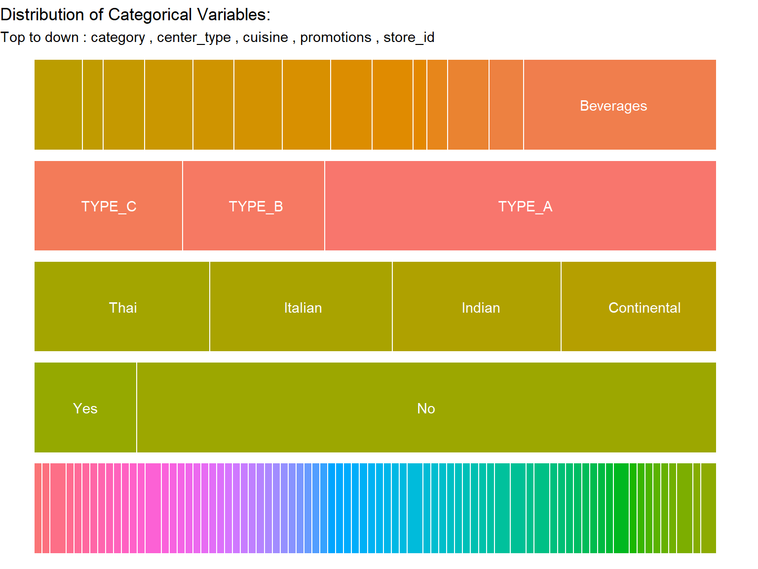
Center Type: Three types, with ‘TYPE_A’ being the most frequent.
Meal Category: Fourteen categories, ‘Beverages’ being the most frequent.
Cuisine: Four types, with ‘Italian’ being the most common.
Code
```{r}#| label: Overview categorical data#| fig-cap: " Distribution of the categorical variables"#| warning: false#| code-fold: true#| fig-width: 8#| fig-height: 6freq_data <- function(df){ df <- as.data.frame(df) results_list <- vector("list", ncol(df) - 1) # Loop through the columns starting from the 2nd column for (i in 2:ncol(df)) { # Store the result of cal_freq(i) in the list results_list[[i - 1]] <- cal_freqx(i, df) } df <- do.call(rbind, results_list) # label bar graph df$vars <- ifelse(df$Freqx > 0.08, as.character(df$Var1), "") return(df)} p <- freq_data(train |> select(-promotion_flag) |> mutate(store_id = as.factor(center_id))) p |> ggplot(aes(x = round(Freqx,2), y = fct_rev(namex), fill = Var1)) + geom_col(position = "fill", color = "white") + scale_x_continuous(labels = label_percent()) + labs(title = "Distribution of Categorical Variables:", subtitle = paste("Top to down :" , unique(p$namex)[2],"," ,unique(p$namex)[1],"," , unique(p$namex)[3],"," , unique(p$namex)[4],"," , unique(p$namex)[5]),y = NULL, x = NULL, fill = "var1")+ guides(fill="none") + geom_text(aes(label = vars), position = position_stack(vjust = 0.5), color = "white")+ theme_void()```
Since we are trying to forecast future demand, we can plot sales and profit of different promotions over time. To do this, we average the data across stores, as this can allow smoothing of the noise to see more of the signal.
Visulization: Effect of Promotion types on Weekly Profit in each store
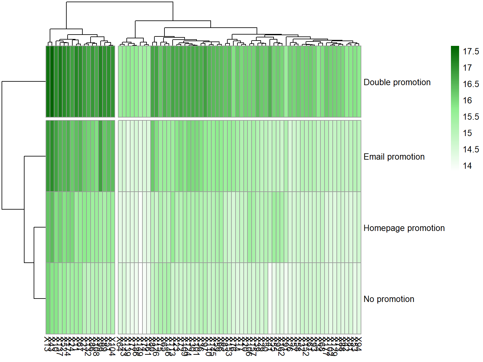
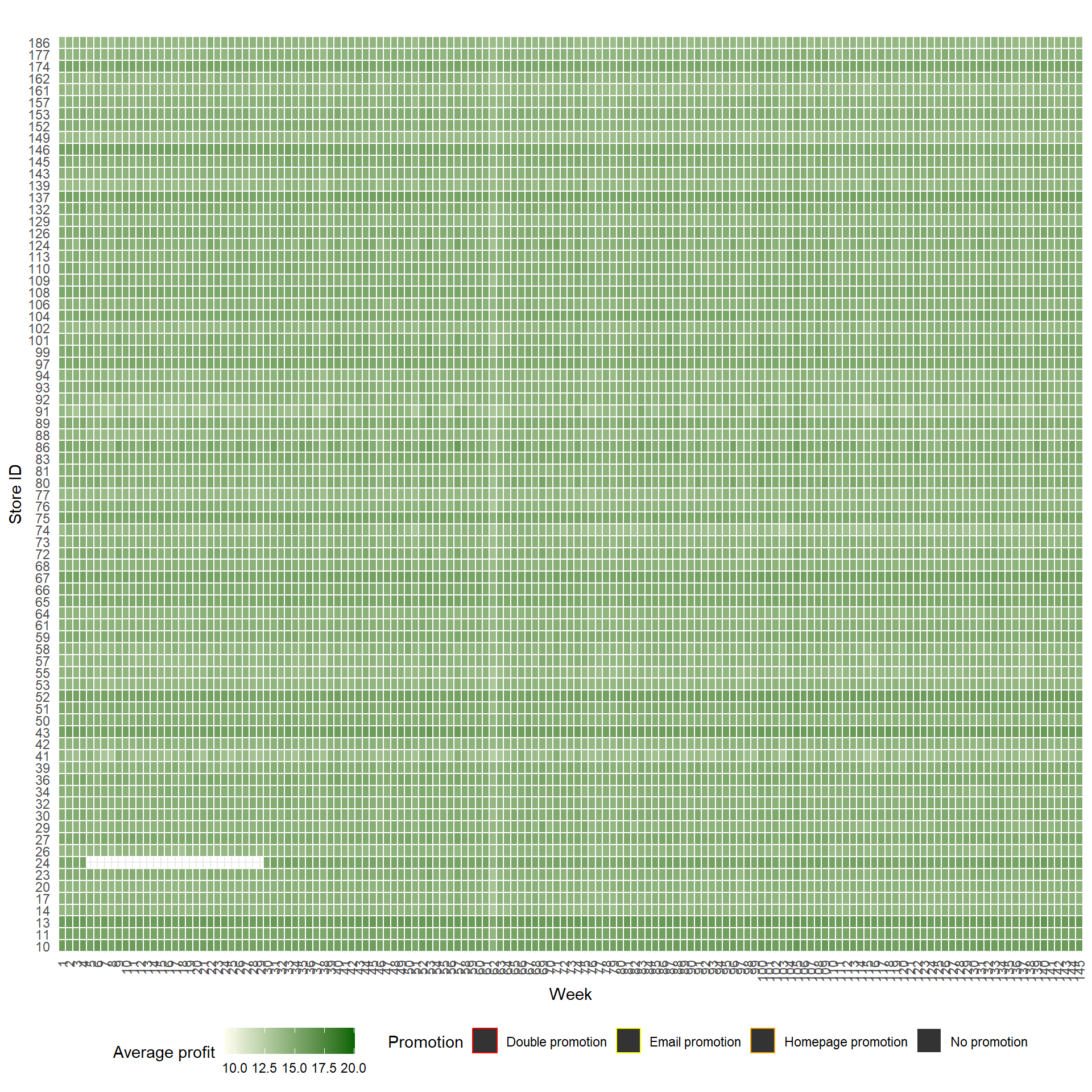
As one of our goals is to identify patterns and correlations between promotion types, individual store performance, and weekly profit trends. We first used a heatmap to help us visualize how well our stores are performing over time and how different promotions impact our profits. Each cell in the heatmap represents the average profit for a specific store (rows) during a specific week (columns). The color intensity (ranging from light to dark green) indicates the magnitude of average profit, with darker greens representing higher profits. The Color bar represents a profit from 10.0 to 20.0. The border of the cell represents the promotion type being carried out in the store for the corresponding week. Namely Promotion, Double promotion, Email promotion, No promotion, and Homepage promotion.
While some stores (e.g., Store IDs around 40-50) consistently show higher profits (darker green), other stores (e.g., Store IDs around 140-150) show consistently lower profits (lighter green). This indicates that the strategies for these stores need a revisit.
Weeks with promotions (identified by the border type) often correlate with higher profits (darker green cells). However, the effectiveness varies.
Patterns in the heatmap suggest potential seasonal cycles, with profit fluctuations happening in waves.
```{r}#| label: Overview profit with heatmap #| fig-cap: "Overview profit with heatmap "#| warning: false#| code-fold: true#| fig-width: 10#| fig-height: 10#--------------- Heatmap overall------train |> group_by(week, promotion_flag, center_id) |> dplyr::summarise(`Average Profit (log2)` = log(mean(profit),2))|> ggplot(aes(x = as.factor(week), y = as.factor(center_id), fill = `Average Profit (log2)`)) + geom_tile(aes(color = promotion_flag), linewidth = 0.5) + # Color outline for promotion scale_fill_gradient(low = "ivory", high = "darkgreen", name = "Average profit") +scale_color_manual(values = c("Double promotion" = "red", "Email promotion" = "yellow", "Homepage promotion" = "orange","No promotion" = "white"), name = "Promotion") + labs(title = " ", #Heatmap of Weekly Profit and Promotions per Store x = "Week", y = "Store ID") + theme_minimal() + theme(legend.position="bottom", axis.text.x = element_text(angle = 90, vjust = 0.5, hjust=1))```
Overview profit with heatmap
Since we are trying to forecast future demand, we can plot sales and profit of different promotions over time. To do this, we average the data across stores, as this can allow smoothing of the noise to see more of the signal.
Visulization: Average Sales and Revenue Over Time
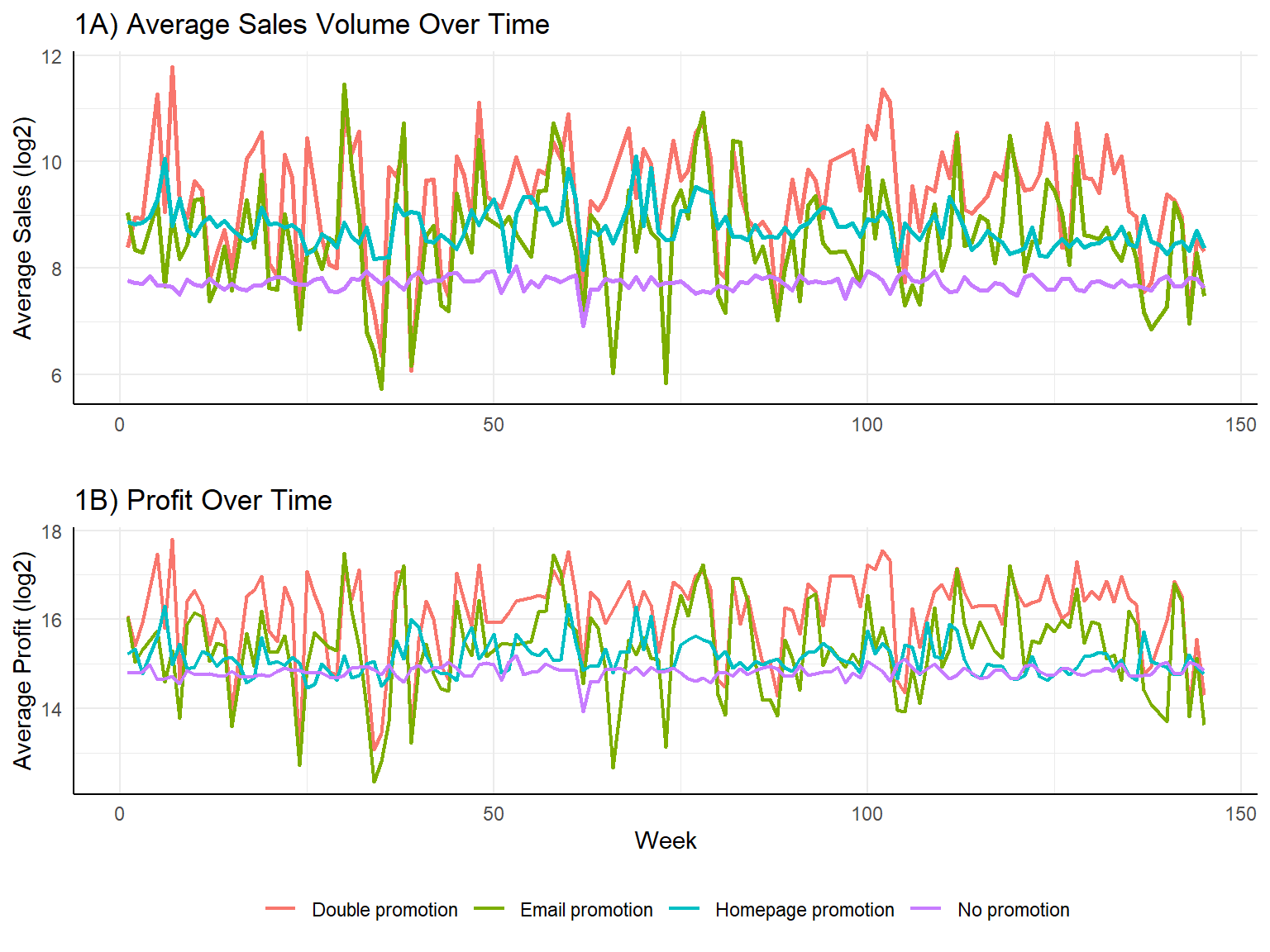
The blue line (No Promotions) is consistently lower and less volatile compared to other lines (Homepage promotion, Email promotion, Double promotion) in figure 1A. This suggests that promotions drive short-term spikes in sales, but the effect is not stable over time. There are frequent peaks and drops, indicating that sales surge when promotions are active but return to normal levels afterward. The profit trend (Figure 1B) mirrors the sales trend, confirming that higher sales during promotions contribute to revenue increases.However, the fluctuations in revenue suggest that while sales increase, revenue might not be growing at the same rate, possibly due to discounting.
Note: The non-promoted sales and revenue (blue line) remain relatively stable over time. The promoted periods exhibit more volatility, meaning promotions may be shifting demand rather than creating long-term sales growth.
Code
```{r}#| label: Time series plots of sales volume and revenue#| fig-cap: " "#| warning: false#| code-fold: true#| fig-width: 8#| fig-height: 6# ---------------------------# 1. Time Series Plot of Sales Volume & Revenue# ---------------------------sales_trend <- train |> group_by(week, promotion_flag) |> dplyr::summarise(average_sales = log(mean(num_orders),2), average_profit = log(mean(profit),2), .groups = 'drop')# Plot Sales Volume Over Time a1 <- ggplot(sales_trend, aes(x = week, y = average_sales, color = as.factor(promotion_flag))) + geom_line(size = 1) + labs(title = "1A) Average Sales Volume Over Time", x = "", y = "Average Sales (log2)", color = "Promotion") + theme_minimal()+ theme(legend.title=element_blank(), legend.position="bottom", panel.background = element_blank())+ theme(axis.line = element_line(color = 'black'))+ guides(color="none")# Plot Revenue Over Time a2 <- ggplot(sales_trend, aes(x = week, y = average_profit, color = as.factor(promotion_flag))) + geom_line(size = 0.8) + labs(title = "1B) Profit Over Time", x = "Week", y = "Average Profit (log2)", color = "Promotion") + theme_minimal()+ theme(legend.title=element_blank(), legend.position="bottom", panel.background = element_blank())+ theme(axis.line = element_line(color = 'black')) grid.arrange(a1, a2, nrow = 2)```
Promotion Effectiveness: Average Weekly Sales & Revenue by Promotion Type
Sales Volume
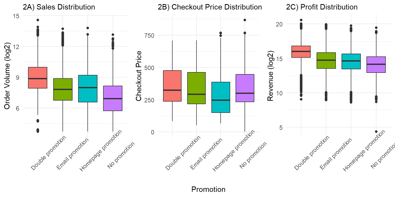
Figure 2A shows how many orders were placed under different types of promotions.The y-axis is in a log scale (log2), meaning the values grow exponentially. The median order volume is highest for double promotions (both email and homepage), followed by homepage promotions, no promotions, and email promotions. The spread (height of the box) indicates variability, with double promotions showing more fluctuation in sales. The presence of numerous outliers at the upper end indicates that some stores experience exceptionally high sales under promotional influence.
Checkout Price
Figure 2B shows the range of prices customers paid at checkout under different promotions. Unlike the sales volume, there is no major difference in checkout price across promotions. There is some right-skewness with outliers, suggesting a small number of high-value purchases, but the overall trend remains stable. This suggests that promotions influence the number of items bought, but not the price per visit.
Profit
Revenue is also log-transformed for better visualization as shown in figure 2C. Similar to the sales volume trend, double promotions generate the highest median revenue, followed by homepage promotions, no promotions, and email promotions. The spread of revenue is wider, meaning revenue varies significantly under all conditions. The presence of high-value outliers suggests that under certain conditions, promotions can lead to exceptionally high revenue generation.
Code
```{r}#| label: Boxplot of sales volume, checkout price and revenue#| fig-cap: " "#| warning: false#| code-fold: true#| fig-width: 8#| fig-height: 4# ---------------------------# Boxplots of Sales with vs. without Promotion# ---------------------------a <- ggplot(train, aes(x = promotion_flag, y = log(num_orders,2), fill = promotion_flag)) + geom_boxplot() + labs(title = "2A) Sales Distribution", x = "", y = "Order Volume (log2)") + theme_minimal()+ theme( legend.position="bottom", plot.title = element_text(size=11), axis.text.x = element_text(angle = 45, vjust = 0.5, hjust=0.2))+ guides(fill="none")b<- ggplot(train, aes(x = promotion_flag, y = checkout_price, fill = promotion_flag)) + geom_boxplot() + labs(title = "2B) Checkout Price Distribution", x = "Promotion", y = "Checkout Price") + theme_minimal()+ theme( legend.position="bottom", plot.title = element_text(size=11), axis.text.x = element_text(angle = 45, vjust = 0.5, hjust=0.2))+ guides(fill="none")c<- ggplot(train, aes(x = promotion_flag, y = log((profit),2), fill = promotion_flag)) + geom_boxplot() + labs(title = "2C) Profit Distribution", x = "", y = "Revenue (log2)") + theme_minimal()+ theme( legend.position="bottom", plot.title = element_text(size=11), axis.text.x = element_text(angle = 45, vjust = 0.5, hjust=0.2))+ guides(fill="none")grid.arrange(a,b,c, ncol = 3)```
Analysis of Meal Popularity During Promotions and No-Promotions
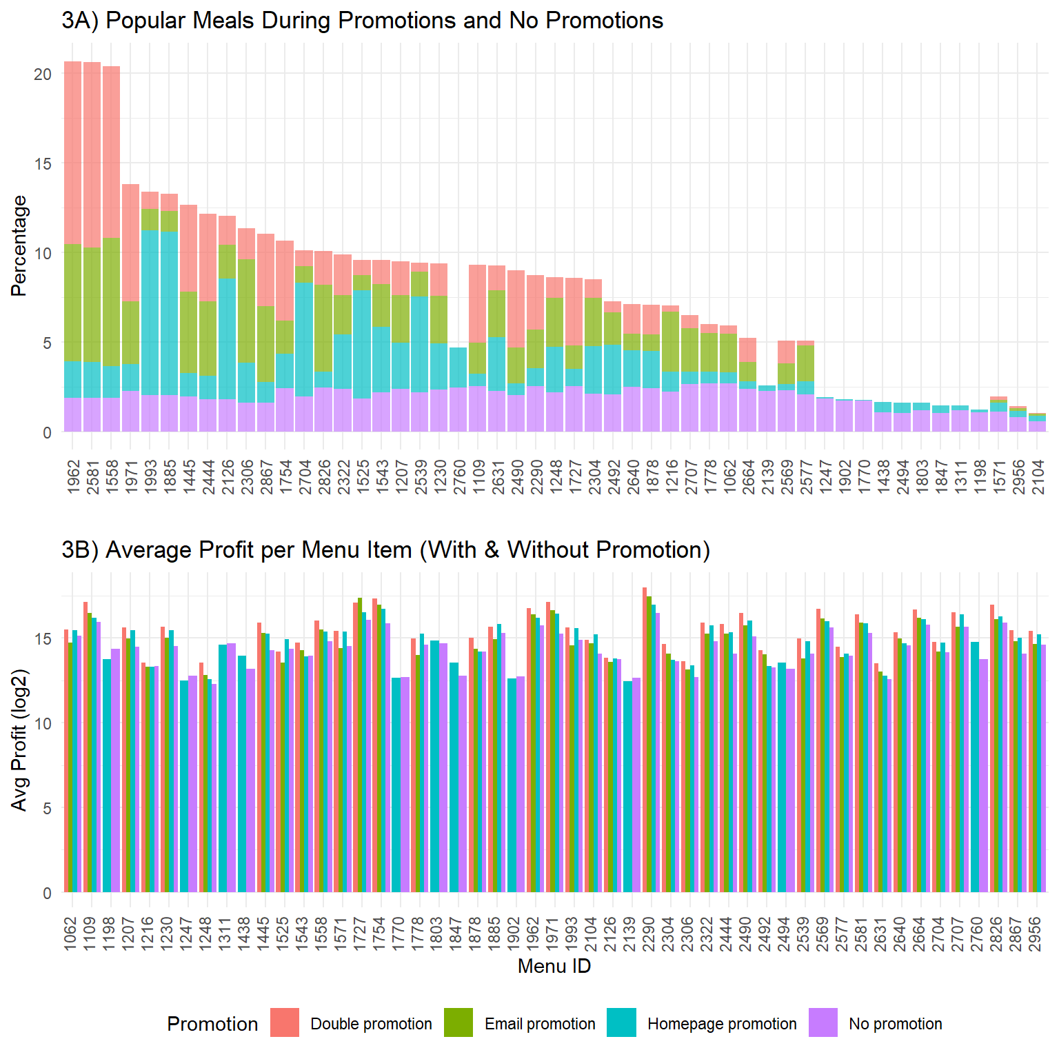
In figure 3A, the Meal IDs are arranged from left to right in descending order based on their overall popularity (total percentage of orders). This visualization helps identify which meals are popular and how promotions influence demand.
Impact of Promotions:
Several meals (especially on the left side of the plot) show a significant increase in order percentage when a promotion is applied. This indicates that promotions can be effective in boosting the popularity of certain meals.For some meals, the Double promotion (email+homepage) or Email promotion seems to have a noticeable impact compared to “No promotion”.
Homepage Promotion Baseline:
Homepage promotion seems to be always present at some level for all meals, which suggests that homepage promotion might be a baseline strategy applied to all meals.
Meal-Specific Promotion Effectiveness:
Some meals respond well to specific types of promotions. For example, Meal ID 1962 sees a significant portion of its orders come from “promotion_flag”. Other meals, like Meal ID 1558, benefits more from “Email promotion”.
Meals with Low Promotion Impact:
On the right side of the plot, the meals have low percentages overall, and the impact of promotions appears to be less significant. This could mean these meals are less popular regardless of promotions, or that the current promotions are not effective for these meals.
Code
```{r}#| label: del Promotions Impact popular items#| fig-cap: " How Promotions Impact checkout price?"#| warning: false#| code-fold: true#| fig-width: 8#| fig-height: 8c1 <- train |> group_by(promotion_flag)|> dplyr::count(meal_id) |> mutate(p = round(100*(n / sum(n)),2))|> select(-n)|> ggplot(aes(x = reorder(factor(meal_id),p,, decreasing = TRUE), fill = promotion_flag)) + geom_bar(aes(y = p), stat='identity', alpha=0.7) + scale_color_manual(values=c('Order Percent'="#d88bb4")) + labs(x = '', y = 'Percentage', title = '3A) Popular Meals During Promotions and No Promotions') + theme_minimal()+ theme(legend.position="bottom", axis.text.x = element_text(angle = 90, vjust = 0.5, hjust=0.5))+ guides(fill="none")c2 <- train|> #filter(meal_id %in% radom_meal)|> group_by(meal_id, promotion_flag) |> summarise(avg_profit = mean(profit), .groups = 'drop')|> ggplot(aes(x = as.factor(meal_id), y = log(avg_profit,2), fill = as.factor(promotion_flag))) + geom_bar(stat = "identity", position = "dodge") + labs(title = "3B) Average Profit per Menu Item (With & Without Promotion)", x = "Menu ID", y = "Avg Profit (log2)", fill = "Promotion") + theme_minimal()+ #guides(fill="none") + theme(legend.position="bottom", axis.text.x = element_text(angle = 90, vjust = 0.2, hjust=0.1))grid.arrange(c1, c2, nrow = 2)```
How Promotions Impact checkout price?
Analysis of Meal Popularity During Promotions and No-Promotions
The average profit per menu item (on the log2 scale) generally falls between approximately 12 and 16 in figure 3B. There’s noticeable variation in average profit across different menu items (identified by their Menu ID). Indeed, we compare the mean profits for No promotion vs. promotins (homepage, email, and homepage+email), the p-value is less than 0.05 from ANOVA test results show promotions substantially impact profits across menu items.
We also see some items are inherently more profitable than others, regardless of the promotion strategy. Certain menu items (e.g., 1248, 1445, 1558) show higher profits under double (homepage and email) promotion, suggesting targeted discounts may work well for these meals. This may indicate that these meals experience higher order volume during promotions, making up for the reduced margin. Since, this isn’t universally true for all menu items. Promotions should be customized per meal item—apply them only where they result in a net positive profit effect.
Code
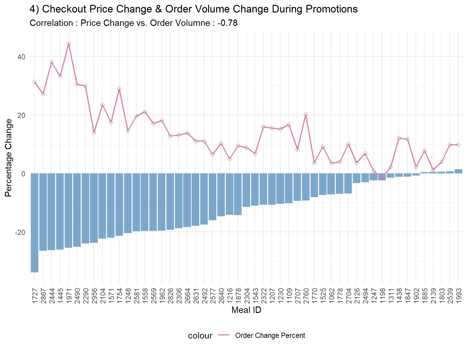
```{r}#| label: Promotions Impact checkout price#| fig-cap: " How Promotions Impact checkout price?"#| warning: false#| code-fold: true#| fig-width: 8#| fig-height: 6# Compute average checkout_price and number of orders before and during promotions for each mealcheckout_price_comparison <- train|> group_by(meal_id, promotions) |> summarise(avg_checkout_price = mean(checkout_price, na.rm = TRUE)) |> spread(promotions, avg_checkout_price)|> mutate(Price_Change_Percent = 100*(Yes - No)/No)comparison_df_order <- train |> group_by(meal_id, promotions) |> summarise(avg_num_orders = mean(num_orders, na.rm = TRUE))|> spread(key = promotions, value = avg_num_orders)|> mutate(Order_Change_Percent = 100*(Yes - No)/No)comparison_df <- left_join(comparison_df_order|> select(meal_id, Order_Change_Percent), checkout_price_comparison|> select(meal_id, Price_Change_Percent), by = "meal_id") # Check correlation between Price_Change_Percent vs Order_Change_Percentcorrelation_po <- round(cor(comparison_df$Order_Change_Percent , comparison_df$Price_Change_Percent , use = "complete.obs"),2)# Plot the resultsggplot(comparison_df, aes(x = reorder(factor(meal_id),round(Price_Change_Percent,2)))) + geom_bar(aes(y = Price_Change_Percent), stat='identity', fill='steelblue', alpha=0.7) + geom_line(aes(y = 0.1*(Order_Change_Percent+4), group=1, color='Order Change Percent'), size=0.8) + geom_point(aes(y = 0.1*(Order_Change_Percent+4), color='darkgray'),shape=21, size=2) + scale_color_manual(values=c('Order Change Percent'="#d88bb4")) + labs(x = 'Meal ID', y = 'Percentage Change', title = '4) Checkout Price Change & Order Volume Change During Promotions', subtitle = paste("Correlation : Price Change vs. Order Volumne :" , correlation_po )) + theme_minimal()+ theme(legend.position="bottom", axis.text.x = element_text(angle = 90, vjust = 0.5, hjust=1))```
How Promotions Impact checkout price?
Keytakeaways
As shown in the heatmap, we know not all stores respond promotions, and some can maintain high profitability without them. We should consider store-specific promotion strategies instead of universal discounting. While double promotions drive the highest sales and revenue, homepage and email promotions individually are not as effective as using both together.
The data shows checkout price per transaction remains stable regardless of the promotion type, meaning the increase in revenue comes from selling more, not from charging more. We can identify stores where promotions significantly boost profits and focus campaigns on those locations. For low-response stores, explore alternative marketing (e.g., bundling, loyalty programs).